AFAI

Sargassum.jl contains tools to generate Sargassum distributions directly from raw Alternative Floating Algae Index (AFAI) data. In brief, AFAI is a quantity derived from satellite observations of certain reflectance bands and is catalogued in ERDDAP. This data can be directly downloaded and managed entirely from Sargassum.jl. Furthermore, distributions are precomputed using default parameters for all available months since 2017.

SargassumDistribution Objects

A SargassumDistribution is defined for a particular year and month. For that month, four aggregated binned distributions are stored, one for each of the weeks defined by the days 1-7, 8-14, 15-21 and 22-28. The value of each bin is equal to the fraction of that month's total coverage. A SargassumDistribution contains the following fields. We describe the fields with minimal jargon here, see SargassumDistribution and the references therein for the full documentation.

• lon: A vector of longitudes (bin edges).

• lat: A vector of latitudes (bin edges).

• time: A DateTime giving the month and year when the distribution was computed.

• coast: A matrix mask defining the location of the coast. The raw AFAI values close to the coast are ignored when calculating the SargassumDistribution since they tend to be inappropriately large.

• clouds: An array mask defining weekly cloud locations, or inavailability of data in general.

• sargassum: An array with dimensions (lon x lat x 4) whose entries give the fractional coverage of Sargassum at each gridpoint and week of the month. Each value is expressed as a percentage of the total coverage in the entire grid in that month, that is, sargassum is a probability distribution on the grid of longitudes, latitudes and weeks. Or, more simply put, we have sum(sargassum) == 1.

Using Precomputed Distributions

Before doing anything else, ensure that the package is loaded into your Julia session,

using Sargassum

These distributions must be downloaded first, which is accomplished simply using the function download_precomputed which downloads each available year's distribution, roughly 5 MB of data per year.

download_precomputed()

This only has to be done once, but can be re-run to download any new available data. All precomputed data is stored in the variable SARGASSUM_DISTRIBUTION_PRECOMPUTED. This is a Dict mapping (year, month) tuples to SargassumDistribution objects. For now, let's visualize the April 2018 weekly distributions using the viz function:

dist_april_2018 = SARGASSUM_DISTRIBUTION_PRECOMPUTED[(2018, 4)]
viz(dist_april_2018, log_scale = true)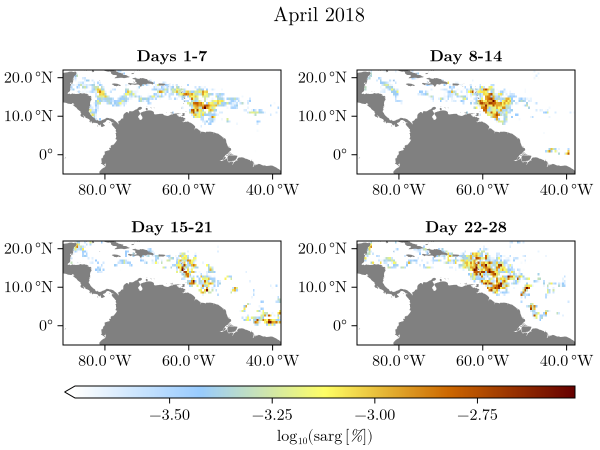

Or, visualize a specific week,

viz(dist_april_2018, 1, log_scale = true)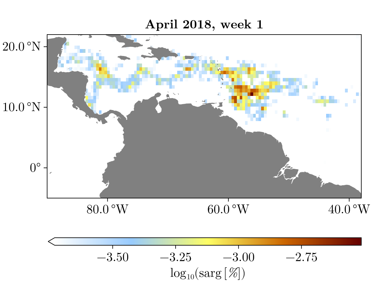

Show the coast and cloud coverage,

viz(dist_april_2018, 1, log_scale = true, show_clouds = true, show_coast = true)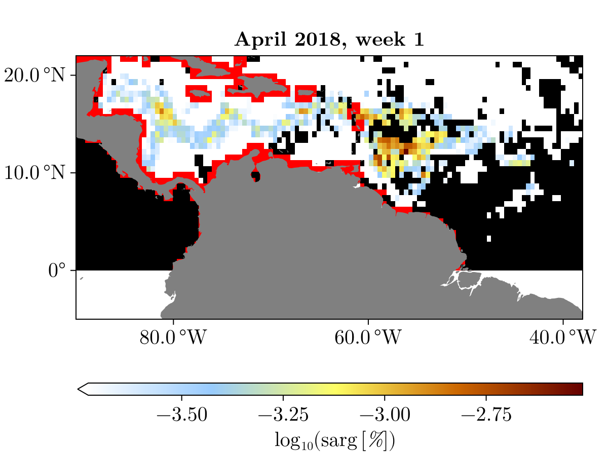

We can examine the distribution numerically. First, we'll read the fields of dist_april_2018 into variables:

lon = dist_april_2018.lon
lat = dist_april_2018.lat
sargassum = dist_april_2018.sargassum

Let's check the monthly coverage in a specific bin:

bin_idx_lon = 70 # the 70'th lon bin
bin_idx_lat = 30 # the 30'th lat bin
bin_centers = (lon[bin_idx_lon], lat[bin_idx_lat])
bin_frac = sargassum[bin_idx_lon, bin_idx_lat, 1] # 1 implies first week
println("The bin centered at $(bin_centers) contains, cumulatively over the first week of April $(100*bin_frac)% of the total Sargassum in the whole of April.")

The bin centered at (-66.8803171641791, 17.515038985392813) contains, cumulatively over the first week of April 0.01943739189300686% of the total Sargassum in the whole of April.

Saving and Loading Distributions

We can save a distribution to a NetCDF file for use elsewhere by applying distribution_to_nc. Multiple distributions can be saved at once.

dist_april_2018 = SARGASSUM_DISTRIBUTION_PRECOMPUTED[(2018, 4)]
dist_may_2018 = SARGASSUM_DISTRIBUTION_PRECOMPUTED[(2018, 5)]
distribution_to_nc([dist_april_2018, dist_may_2018], "dist_april_may_2018.nc")

A saved set of SargassumDistributions can be loaded later via

SargassumDistribution("dist_april_may_2018.nc")

Note that when a SargassumDistribution is loaded in this manner, what is actually returned is a Dict mapping (year, month) tuples to SargassumDistribution objects, in the same manner as SARGASSUM_DISTRIBUTION_PRECOMPUTED. This applies even if the NetCDF file only contains a single SargassumDistribution.

Raw AFAI Data

Raw AFAI data can be downloaded using the function download_raw_afai. The signature of download_raw_afai is

download_raw_afai(year, month_spec; force)

year is the desired year, month_spec can be one of the following

• an integer between 1 and 12: download the data from the corresponding month

• a vector of integers each between 1 and 12: download the data from all of the corresponding months

• omitted: download the data for every month in the given year

If force = true, the data is downloaded even if it already has been. Let us download the data for April, 2018.

download_raw_afai(2018, 4)

The paths to the raw data are stored in AFAI_DOWNLOADED_PATHS, which is a Dict mapping (year, month) pairs to the path of the downloaded data. In this case, AFAI_DOWNLOADED_PATHS[(2018, 4)] will return the path to the data we just downloaded. This can be directly loaded into an AFAI object, which holds the data itself and the AFAIParameters that define how the distribution is computed. Refer to the full documentation for AFAIParameters for more information regarding these parameters. For now, we will use the default values and hence AFAIParameters() will be a sufficient constructor. The signature for an AFAI object is

AFAI(filename, params)

where filename is the NetCDF file that holds the raw AFAI data (assumed to have been downloaded using download_raw_afai) and params is an AFAIParameters. Therefore, we have

filename = AFAI_DOWNLOADED_PATHS[(2018, 4)]
params = AFAIParameters()
afai = AFAI(filename, params)

AFAI[10138534 pixels, Lon ∈ (-98.0, -38.0), Lat ∈ (0.0, 38.0), April 2018]

This can also be visualized using viz,

viz(afai, thresh = 0.9) # only look at the data in the 90th percentile.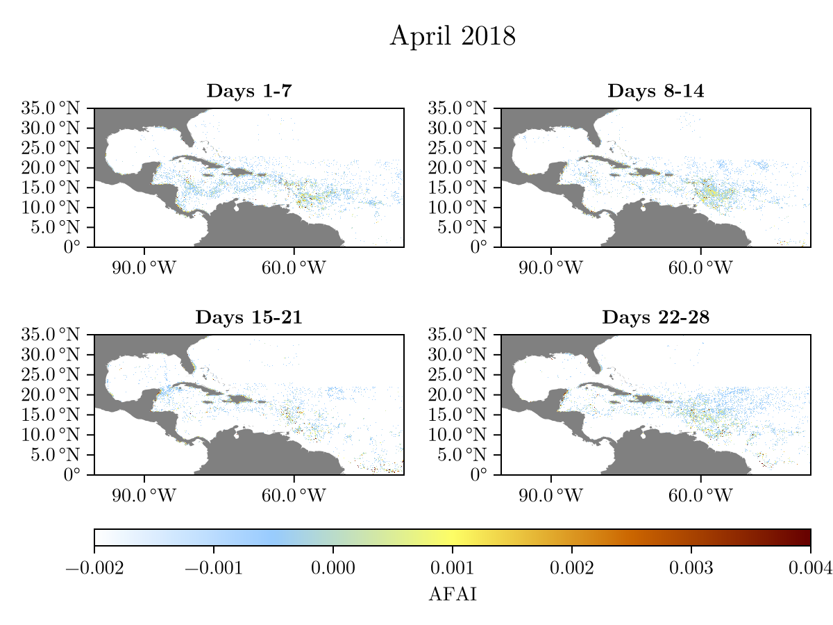

Refer to remove_raw_afai to remove downloaded data.

Constructing Your Own SargassumDistributions

The highest level function for constructing a custom SargassumDistributions is sargassum_distribution. The signature of sargassum_distribution is

sargassum_distribution(year, month_spec, outfile; params)

where year and month_spec are defined identically as in the download_raw_afai function seen previously and outfile is a NetCDF file to which the computed SargassumDistribution(s) are written. The optional argument params is an AFAIParameters object that controls the specifications of how the distribution is computed from the raw AFAI data.

The following command will (1) download the raw AFAI data for April 2018 if it has not already been downloaded (if you ran download_raw_afai earlier, this is automatically recognized and the download is skipped) and (2) compute the SargassumDistribution using default AFAIParameters and finally (3) write the result to "dist_april_2018_downloaded.jl".

Tip

Computing a SargassumDistribution may take several minutes, but the process is automatically parallelized when multiple threads are available. Start Julia with julia --threads=auto instead of julia in order to take advantage of this. Run Threads.nthreads() in the REPL to see how many threads are available in your instance of Julia; as long as at least 4 are available, the computation will be efficient.

sargassum_distribution(2018, 4, "dist_april_2018_downloaded.jl")

This distribution can be examined using SargassumDistribution("dist_april_2018_downloaded.jl") and plotted as done previously.