Simulation

Sargassum.jl contains full physics and biology simulation for Sargassum clumps. To follow along with this tutorial, ensure that Sargassum.jl has been installed with the default interpolants as described in Getting Started.

First Steps

Before doing anything else, ensure that the package is loaded into your Julia session,

using Sargassum

The highest level function in the package is simulate, which takes one mandatory argument, a RaftParameters object. The general plan is therefore to build the RaftParameters object that defines the problem we want to solve. Then, we will simply invoke simulate.

To get up and running as fast as possible, we can use QuickRaftParameters to generate our RaftParameters.

rp = QuickRaftParameters()

 RaftParameters
ICS = InitialConditions[time ∈ (2018-04-13T00:00:00, 2018-04-15T00:00:00), n_clumps = 25, lon/lat ∈ (-55.0, -50.0) × (5.0, 10.0)]
Clumps = ClumpParameters[α = 0.005427, τ = 0.01864, R = 0.7883, Ω = 6.283, σ = 0.0]
Springs = BOMBSpring[A = 1.0, L = 151.9592522325231]
Connections = ConnectionsNearest
GrowthDeath = ImmortalModel

Observe that RaftParameters prints out information about its contents, which we will discuss further later. For now, note that the initial conditions inform us that we are simulating from April 13, 2018 to April 15, 2018 with 25 clumps. A "clump" is a discrete chunk of Sargassum. In the language of Sargassum.jl, a "Raft" is a collection of any number of clumps (including a single clump). Each clump in a raft shares a number of physics parameters via ClumpParameters. For now, we will proceed with the simulation.

rtr = simulate(rp)

RaftTrajectory[25 trajectories, 21 times]

The output of simulate is a RaftTrajectory object. This holds all of the information about each clump's trajectory during the simulation. The easiest way to interpret the results of the simulation is to create a plot. We can use the viz function to get a plot with some default arguments already chosen for us.

viz(rtr, limits = (-60, -45, 0, 15)) # limits = (lon_min, lon_max, lat_min, lat_max)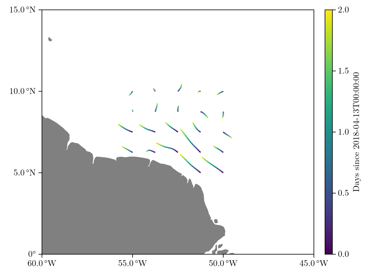

We see a small amount of movement off the coast of Brazil. Suppose we want to save this data for future analysis; for this we can use the rtr2mat function to generate a .mat file which can be read in MATLAB, Python, Julia and other languages with the appropriate package.

rtr2mat(rtr, "first_steps.mat")

Run pwd() to see your current working directory, and find the file first_steps.mat.

Building your own RaftParameters

Introduction to RaftParameters

The "atom" of a Sargassum simulation is called a clump such that a clump is qualitatively a handful of Sargassum. Each clump has identical physics parameters and is modeled as a hard sphere via the Maxey-Riley equations. Sets of clumps are referred to as rafts and are joined together by springs that model interaction forces. Clumps grow and die by biological effects and may die when reaching land. The RaftParameters collects all of this information.

We now provide a walkthrough of the construction of a RaftParameters object. We will essentially recreate Examples.QuickRaftParameters() to show how this is done. The signature of the basic RaftParameters constructor is

RaftParameters(; ics, clumps, springs, connections, gd_model, land, n_clumps_max, geometry = true, fast_raft = false)

Each of these kwargs are defined as follows. We describe the fields with minimal jargon here, see RaftParameters and the references therein for the full documentation.

• ics: The initial conditions of the simulation, including coordinates and simulation time span. Contained in an InitialConditions.

• clumps: Physics parameters defining each (identical) clump; buoyancy, windage etc. Contained in a ClumpParameters object.

• springs: Spring parameters defining each (identical) spring. Contained in a AbstractSpring object.

• connections: Connections defining how the clumps are connected by the springs. Contained in an AbstractConnections object.

• gd_model: A model controling how clumps grow and die due to biological effects. Contained in an AbstractGrowthDeathModel object.

• land: A land model; how clumps should behave when reaching land. Contained in an AbstractLand object.

• n_clumps_max: The maximum number of clumps allowed to exist across the entire simulation. Should be a positive integer.

• geometry: A Boolean flag. If true, corrections are applied to account for the spherical geometry of the Earth. The default value of this is true and we will leave it alone for now.

• fast_raft: A Boolean flag that controls whether a "total" interpolant is created before the integration to save time on multiple evaluations. This is technical, and we omit the discussion for now. The default value of this flag is false and we leave this set as is.

Defining each argument

Click the relevant tab to see how each argument is constructed.

We construct ics, an InitialConditions object. There are several constructors for different situations, but to create a rectangular arrangement, the appropriate constructor is

InitialConditions(t_span, x_range, y_range; to_xy)

The integration time span is controlled by t_span, of the form (t_initial, t_final) and we want to integrate from April 13, 2018 to April 15, 2018. We can use Julia's built-in Dates module to easily define times as DateTime(year, month, day):

using Dates
t_initial = DateTime(2018, 4, 13)
t_final = DateTime(2018, 4, 15)
t_span = (t_initial, t_final)

Next, we need x_range and y_range which can be created quickly using range(start, stop; length). Our example consisted of a 5 x 5 grid of clumps off the coast of Brazil. We can recreate this via

x_range = range(-55.0, -50.0, length = 5)
y_range = range(5.0, 10.0, length = 5)

Note that we have defined our ranges in terms of longitude/latitude. The optional argument to_xy of InitialConditions should therefore be set to true to automatically convert these spherical coordinates to equirectangular coordinates.

ics = InitialConditions(t_span, x_range, y_range, to_xy = true)

InitialConditions[time ∈ (2018-04-13T00:00:00, 2018-04-15T00:00:00), n_clumps = 25, lon/lat ∈ (-55.0, -50.0) × (5.0, 10.0)]

While we're here, we can define the maximum number of clumps we want to allow. This example contains no biological effects, so the maximum number of clumps will simply be equal to the initial number of clumps, 25.

n_clumps_max = 25

Application

Now that all the appropriate arguments are defined, we simply use the RaftParameters constructor.

rp = RaftParameters(
    ics = ics,
    clumps = clumps,
    springs = springs,
    connections = connections,
    gd_model = gd_model,
    land = land,
    n_clumps_max = n_clumps_max
)

 RaftParameters
ICS = InitialConditions[time ∈ (2018-04-13T00:00:00, 2018-04-15T00:00:00), n_clumps = 25, lon/lat ∈ (-55.0, -50.0) × (5.0, 10.0)]
Clumps = ClumpParameters[α = 0.005427, τ = 0.01864, R = 0.7883, Ω = 6.283, σ = 0.0]
Springs = BOMBSpring[A = 1.0, L = 151.9592522325231]
Connections = ConnectionsNearest
GrowthDeath = ImmortalModel

And now we can simulate and plot as earlier:

rtr = simulate(rp)
viz(rtr, limits = (-60, -45, 0, 15))

Comparing this to our earlier example, we see that they are indeed identical.

Advanced RaftParameters Construction

An easy way to see the available options for a certain RaftParameters object is to use the subtypes command. For example, the connections argument is an AbstractConnections and we have

subtypes(AbstractConnections)

4-element Vector{Any}:
 ConnectionsFull
 ConnectionsNearest
 ConnectionsNone
 ConnectionsRadius

Then, we can examine the documentation of any of these by typing ? to access the help> prompt followed by the desired name. For example, ConnectionsNearest reads

Sargassum.ConnectionsNearest Type

struct ConnectionsNearest

A connection type such that every clump is connected to a number of its nearest neighbors.

Fields

• neighbors: The number of nearest neighbors each clump should be connected to.

Constructors

ConnectionsNearest(n_clumps_max, neighbors)

source

In this case, we see that ConnectionsNearest assigns connections between a clump's k-nearest neighbors and has the constructor ConnectionsNearest(n_clumps_max, neighbors).

Refer to the simulation API for further information on the built-in options and refer to the custom physics and custom biology sections for tutorials on building your own objects.