Interpolants

Sargassum.jl comes with 7 global variables (technically Refs) that store computed interpolants. These are WATER_ITP, WIND_ITP, STOKES_ITP, WAVES_ITP, NUTRIENTS_ITP, TEMPERATURE_ITP and LAND_ITP. These variables are initially undefined but default interpolants for the year 2018 are available for download directly from within the package. These default interpolants are useful for testing purposes and for simulations, but are not strictly required.

Interpolants are InterpolatedField objects. Refer to the InterpolatedField documentation for the full details of this object. Here we will use the interfacing functions that will allow us to avoid dealing with the details.

Constructing the Default Interpolants

The raw data that the interpolants depend on must first be downloaded, and then the interpolants themselves must be constructed. This process only needs to happen once. The main function to accomplish this is itps_default_construct. This function takes no argument, but has a keyword download, such that if download = true is passed, the raw data will be downloaded. If the data have already been downloaded, itps_default_construct will rebuild the interpolants. An easy way to check if you have the default interpolants loaded is to simply run WATER_ITP,

WATER_ITP

Base.RefValue{InterpolatedField}(InterpolatedField
Dimensions = Fields = lon/lat ∈ (-100.9, -39.12) × (0.125, 39.88)]
time ∈ (2018-01-01T00:00:00, 2018-12-31T00:00:00))

Tip

Did you run WATER_ITP and get no output? Try running itps_default_construct(). If this doesn't work, then run itps_default_construct(download = true), which will download roughly 1.2 GB of data.

We see that several useful pieces of information have been printed out that let us know the variables, fields and limits that define the interpolant. The other interpolants can be inspected in the same way.

Inspecting Interpolants

The primary elements of an InterpolatedField are dimensions (things like x, y and t) and fields (things like velocity and temperature). We can use dims, fields and boundary to quickly inspect these.

dims(WATER_ITP)

3-element Vector{Tuple{Symbol, Unitful.Unitlike}}:
 (:x, km)
 (:y, km)
 (:t, d)

fields(WATER_ITP)

5-element Vector{Tuple{Symbol, Unitful.Unitlike}}:
 (:u, km d^-1)
 (:v, km d^-1)
 (:DDt_x, d^-2)
 (:DDt_y, d^-2)
 (:vorticity, d^-2)

boundary(WATER_ITP)

(-100.9, -39.12, 0.125, 39.88, "2018-01-01T00:00:00", "2018-12-31T00:00:00")

We see each dimension and field along with its units. The boundary function prints its output in the form (lon_min, lon_max, lat_min, lat_max, time_min, time_max) for time-dependent fields and (lon_min, lon_max, lat_min, lat_max) for time-independent fields.

Tip

Why does boundary print longitudes and latitudes if dims indicates that the fields :x and :y have units of km? The answer is that InterpolatedFields are assumed to the in equirectangular coordinates, since these are the coordinates expected by the differential equations we eventually integrate. However, these coordinates are hard to parse, so they are converted to spherical coordinates before printing.

We can access the actual value of dimensions and fields using the dim and field functions, respectively. The first argument to each is the InterpolatedField and the second argument is one of the Symbols in the output of dims or fields.

x_water = dim(WATER_ITP, :x)
y_water = dim(WATER_ITP, :y)
t_water = dim(WATER_ITP, :t)

6575.0:1.0:6939.0

u_water = field(WATER_ITP, :u)
size(u_water) # just print the size, since the actual array is huge

(248, 160, 365)

Note that the order that the dimensions appear in in the output of dims is the same order that they are defined for the fields. Here, field(WATER_ITP, :u) is the interpolant of a three dimensional array where the first dimension corresponds to :x:, the second to :y and the third to :t.

The interpolant fields can be called like functions.

pt = x_water[10], y_water[10], t_water[10]
u_water(x_water[10], y_water[10], t_water[10])

-42.20153086406751

Finally, a field from an InterpolatedField can be quickly visualized with viz,

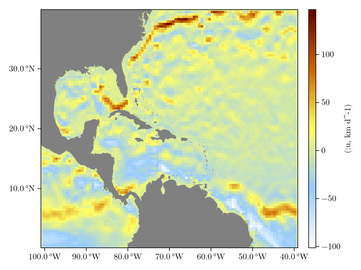
viz(WATER_ITP, :u)

Building Your Own Interpolants

Here we will describe the functions that allow the construction of interpolants from raw data. We will recreate WIND_ITP from scratch to see how this is done. In order to follow this tutorial, the default interpolants should be downloaded. The first step is to locate the NetCDF file that contains the data. For this we use the variable Sargassum._ITPS_RAW_SCRATCH which is generally not intended to be user-facing, but suffice to say that the following command will retrieve the path to the required NetCDF field.

infile = joinpath(Sargassum._ITPS_RAW_SCRATCH.x, "wind.nc")

"/home/runner/.julia/scratchspaces/022a0cfc-64d6-4a4c-8da6-19b349a396b3/_ITPS_RAW_SCRATCH/wind.nc"

Now, we will use the Julia package NetCDF to inspect this file via the ncinfo function.

using NetCDF
ncinfo(infile)

##### NetCDF File #####

/home/runner/.julia/scratchspaces/022a0cfc-64d6-4a4c-8da6-19b349a396b3/_ITPS_RAW_SCRATCH/wind.nc

##### Dimensions #####

Name                                                Length
--------------------------------------------------------------------------------
latitude                                            161
time                                                365
longitude                                           241

##### Variables #####

Name                            Type            Dimensions
--------------------------------------------------------------------------------
u10                             SHORT           longitude latitude time
latitude                        FLOAT           latitude
time                            INT             time
longitude                       FLOAT           longitude
v10                             SHORT           longitude latitude time

##### Attributes #####

Variable            Name                Value
--------------------------------------------------------------------------------
global              history             2023-10-26 20:53:02 GMT by grib_to_net..
global              Conventions         CF-1.6
u10                 missing_value       -32767
u10                 units               m s**-1
u10                 add_offset          -0.7626114861385587
u10                 long_name           10 metre U wind component
u10                 scale_factor        0.0009157213005548016
u10                 _FillValue          -32767
latitude            units               degrees_north
latitude            long_name           latitude
time                units               hours since 1900-01-01 00:00:00.0
time                calendar            gregorian
time                long_name           time
longitude           units               degrees_east
longitude           long_name           longitude
v10                 missing_value       -32767
v10                 units               m s**-1
v10                 add_offset          1.4802321238623486
v10                 long_name           10 metre V wind component
v10                 scale_factor        0.0009004983690528532
v10                 _FillValue          -32767

This prints a lot of information, and we should take particular note of

The names and units of the dimensions

• latitude in degrees north

• longitude in degrees east

• time in hours since 1900-01-01

The names and units of the fields

• u10 in m/s

• v10 in m/s

Click the tabs to see the steps of the construction.

To begin construction of the interpolant, we start with a GriddedField whose job it is to hold the raw data and variable definitions before the actual interpolation in performed. The GriddedField constructor takes a single argument, the number of dimensions of the field in question. In this case, 3 since we have a time-dependent field.

using Unitful
using Dates
gf = GriddedField(3)

Loading Your Own Interpolants

We will use the interpolant created in the previous section as an example, i.e. we assume there is a file wind_test_file = "WIND_ITP_TEST.jld2" in the current working directory. We can load the interpolant into memory using load(file, variable) from JLD2.

wind_itp_test = load(wind_test_file, "WIND_ITP")

To "activate" this interpolant, we must replace the current wind interpolant. This is accomplished using [update_interpolant!],

update_interpolant!(WIND_ITP, wind_itp_test)